When you start out with machine learning and AI you will learn very quickly that there's a lot of math involved.
All this math is very hard to understand, especially if you have a background in software engineering rather than
statistics. Most of the stuff you will find on the internet assumes that you know your statistics, which you probably don't.
In this series I will invite you along on my personal AI trip along some very cool algorithms and seriously hard topics.
I will explain them as simple as I can so you too can start to use machine learning and deep learning in your daily work.
In this series I will address the following topics:
- What is a gradient descent algorithm?
- Which algorithm should I use for what?
- How do I know whether my ML model is any good?
- What exactly is a neural network and why should I care?
- I don't think I have enough data, what can I do?
I will add more topics in the next months as we go along.
Introduction
One of the hardest things in machine learning I've found is how the computer actually learns when you apply a machine learning algorithm.
There are gradient descent algorithms being thrown around like there's no tomorrow, but what are they?
In this post I will explain what a gradient descent algorithm is, by starting with a basic explanation of linear regression
and then slowly working up to the gradient descent algorithm and what it does in relation to the linear regression algorithm.
Define a model
Most of the time we can define the output of a computer algorithm by implementing business rules for our problem space.
These business rules include formulas and conditions under which these formulas work. However, sometimes that doesn't solve
the problem. This is the case when we don't know the exact formula that correctly describes the solution for a problem.
For example, if you want to predict the price of a house you could define a formula yourself. But it will most likely
not be very useful. That's because the price of a house is influenced by a lot of factors. Also, there's a hidden relationship between
all of these factors that ultimately determine the price of a house.
The only way to make a sensible prediction is by letting the computer train itself to find the hidden relationship between features.
Instead of defining the complete formula manually you define a model that the computer then can train.
To predict the price of a house you can define a function that takes in the features of a house and predicts a price by multiplying the values
for the features with a set of weights that simulate the relationship between the features.
$$\hat{y}=w_1x_1+w_2x_2+w_3x_3+...+w_nx_n$$
$w_1...w_n1$ are unknown in this case since we're searching for the hidden relationship between the various variables.
We're going to optimize the weights in such a way that the difference between our predictions and the actual price of a house is minimal as possible.
Typically when you want to model something like the predicted price of a house you use a model called linear regression.
Linear regression is defined as a function of the form
$$y = b+wx$$
This can get more complicated, but for this post I will stick to the simple form. The variable x we know, this is the input.
The variable y is the output we want to predict. The variables $b$ and $w$ are unknown. Typically we call the variable $b$ the bias
and the variable $w$ the weight of the input.
Define an objective
In order to find the ideal weight and bias we have to first define an objective for the algorithm. The objective is a function that calculates
the error rate. Basically, how far off are we with a given set of weights. The goal is to minimize the output of this function.
For our function we want to know the difference between the real output and the predicted output.
We want to use the average of these errors so that we learn how far off we are in general. So we could define the objective function (or loss function)
as follows:
$$error=\frac{1}{N}\sum_{i=1}^Ny_i-\hat{y_i}$$
The variable $\hat{y}$ is the predicted price, the variable $y$ is the actual price of the house. We sum all the differences and multiply them by $\frac{1}{N}$
to calculate the average error.
This looks okay, but there's a problem. When there's one input that predicted with an error of 5 and another with an error of -5 you get an error
rate of exactly zero. Thus our weights are optimal, but that's not correct as you can see.
To account for this problem you can square the error values. This causes to all the price difference to be positive. It also punishes the computer
for large differences between predictions and actual values.
$$error=\frac{1}{N}\sum_{i=1}^N(y_i-\hat{y_i})^2$$
Note: Although we went over the loss function in great detail, you will often use standard loss functions that others have come up with before.
The trick is to know which loss function to use. In the next posts in this series I will show you some more loss functions that are typically
used.
Optimizing the weights
The goal for the computer is to make the error rate as small as possible. You could argue that you can put in random numbers again and again to find the
right solution since there's no way you know the actual values. But that would take an infinite number of hours. That's because you cannot know when you've
reached the optimal value for the weights.
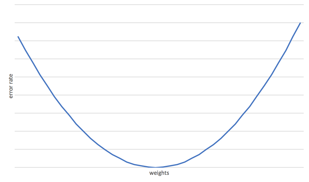
There is however a relationship between the value of the loss function and the weights. When you draw a graph of the weights related to the
output of the loss function you will see that it has a typical shape.

This gave the mathmeticians that came up with gradient descent an idea. The error rate is the function of the weights in relationship to the
inputs that we know. You could, instead of random guessing use derived functions to find the rate of change to the weights at each point in the
chart.
When you know the gradient of the weights you can iteratively modify them so that with every iteration you move closer to their optimal value.
Now that all sounds great, but how does it work? For this I need to introduce a bit more math than before.
The first step in calculating the gradient is to create a partially derived function for each variable that we want the gradient for.
We need to find the gradient for a specific variable in our loss function. So instead of creating a regular derived function that you normally
use to find a gradient in a line, we need to derive the loss function for the weights that we want the gradient of.
To keep things simple, let's try to find the gradients for the bias and weight in the following loss function:
$$error=\frac{1}{N}\sum_{i=1}^N{(y-(b + wx))^2}$$
Note: I have replaced the predicted value $\hat{y}$ for the formula that calculates this value.
You can come up with the following partially derived functions:
$$\frac{\partial}{\partial{w}}=\frac{2}{N}\sum_{i=1}^N-x_i(y_i-(b + wx_i))$$
$$\frac{\partial}{\partial{b}}=\frac{2}{N}\sum_{i=1}^N-(y_i-(b + wx_i))$$
Let's go over the equations in more detail so you know what is going on. A partially derived function only calculates the gradient for one
variable at a time. The rest is left as is. You can recognize this by the division at the left hand side of the equation. The denominator tells you
it's a derived function. The divisor then says it's a derived function for a particular variable. The right hand side of the equation is the derived
function.
Note: I understand that if you don't have a background in math the above formulas are magic.
Manually creating derived functions can be a fun excercise, but I wouldn't recommend it. Instead, let the computer
fix this problem. Tools like tensorflow, Microsoft Cognitive Toolkit and Keras automatically create derived functions
for loss functions you provide them. Much better right?
When you apply the derived functions in code , you will get a small piece of code that can iteratively determine the correct weights.
Let's look at some code for this:
def step_gradient(x, y, weight, bias, learning_rate):
    temp_weight = 0
    temp_bias = 0

    N = float(x.shape[0])

    for j in range(x.shape[0]):
        temp_bias += - (2 / N) * (y[j] - ((weight * x[j]) + bias))
        temp_weight += -(2 / N) * x[j] * (y[j] - ((weight * x[j]) + bias))

    new_weight = weight - (learning_rate * temp_weight)
    new_bias = bias - (learning_rate * temp_bias)

    return new_weight, new_bias


def gradient_descent(x, y, bias, weight, learning_rate, iterations):
    for i in range(0, iterations):
        new_weight, new_bias = step_gradient(x, y, weight, bias, learning_rate)

        weight = new_weight
        bias = new_bias

    return weight, bias
The gradient descent algorithm in this sample has two functions. First there's the gradient_step function
and second there's the gradient_descent function. The gradient_descent function iteratively calls the
gradient_step function with the current weights and inputs. The gradient_step function takes the original
weights and inputs. It then calculates the gradients for all the points in the dataset x and uses these
gradients to update the bias and weight.
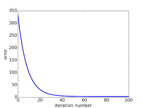
By running this algorithm a number of times you will see that the weights decrease until they reach their optimal value.

At first the the gradient is very steep, this means that we're learning fast. Near the end of the iterations you will notice that the gradient is not so steep anymore. This means we're near our goal. When it reaches the optimal value isn't something that you can know up front.
You have to decide for how long you want to gradient descent algorithm to run. Typically you run the algorithm for about 1000 to 10000 iterations to
ensure that you've reached the optimum values.
What does the learning rate have to do with this algorithm?
You could argue that updating the gradient with the delta should get you there faster than updating it in small steps using the learning rate.
Remember, we're walking a gradient. If you use big steps you will get down fast. But the line in the error rate chart also goes up after we've reached the
optimum value. This is the point beyond which there's no use in updating the weights, since we're only getting worse.
A small learning rate prevents your optimization from overshooting its goal. However, if you make the learning rate too small you
will not reach your goal in time. Typically you will have a learning rate between 0.01 and 0.001.
Balancing the learning rate is also something that the computer does not do for you. You have to experiment and find the right learning rate
for the function you're trying to optimize.
Summary
The gradient descent algorithm is method that uses the gradients of unknown variables to change them iteratively so that we have
a guarantueed method of reaching the optimal values for a set of unknown variables in a function.
As you can imagine, machine learning involves mostly finding optimal values for unknown factors in equations.
Because that is basically what you want the computer to find out when you want to predict something based on
input that you've seen before.
The process of learning to predict an output, whether that is a class (positive, negative) for a set of inputs or a continuous value
such as the predicted price of a house, it all works like this:
- Define a model
- Define a loss function
- Minimize the loss function using gradient descent
In the next posts you will learn that this trick is used practically everywhere even in neural networks which are
quite a bit harder than linear regression.
I hope you liked this post. Leave a comment if you have any questions or comments.